[ML Study Jam in DSC Sookmyung] Intro to Machine Learning(Kaggle)

2021.03.28(일) 작성
www.kaggle.com/learn/intro-to-machine-learning

 

Basic Data Exploration

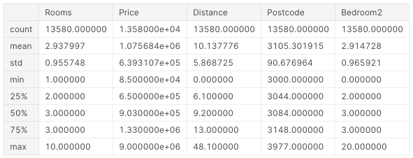
데이터 탐색을 위해 pandas 라이브러리 이용. read_csv() 를 통해 csv 파일을 읽어들일 수 있으며, describe() 메서드로 각 attribute에 대한 통계값을 확인할 수 있다.

import pandas as pd

file_path = '../input/melbourne-housing-snapshot/melb_data.csv'
data = pd.read_csv(file_path)
data.describe()

실행 결과는 다음과 같다.

 

데이터로부터 subset 추출

한 column만 가져오기

dot-notation으로 해당 column에 대한 Series(column 1개만 있는 Dataframe)를 가져올 수 있다.

y = data.Price

여러 column 가져오기

가져오려 하는 feature들을 담은 배열을 만들어 여러 column을 가져올 수 있다.

features = ['Rooms', 'Bathroom', 'Landsize', 'Lattidute', 'Longtitude']
X = data[features]
X.describe()

 

모델 빌드하기

scikit-learn 을 사용할 것이며, sklearn 라이브러리를 통해 사용할 수 있다.

모델을 빌드하고 사용하는 과정은 다음과 같다:

1. Define: 어떤 모델을 만들 것인가?(decision tree, SVM 등)
2. Fit: 준비한 데이터로부터 패턴을 파악한다.
3. Predict: 말 그대로 예측한다.
4. Evaluate: 모델의 예측 정확도를 판단한다.

scikit-learn을 통해 decision tree 모델을 만들고 예측하는 예제를 살펴보자.

from sklearn.tree import DecisionTreeRegressor

# Define
model = DecisionTreeRegressor(random_state=1)
# Fit
model.fit(X, y)

DecisionTreeRegressor 에서 random_state key에 대해 임의의 수를 지정할 수 있다. 많은 머신러닝 모델은 트레이닝 과정에서 임의성을 허용하는데, 같은 random_state 값을 지정한 실행에 대해서 같은 결과가 도출됨이 보장된다. 어떤 수라도 사용할 수 있으며, 모델의 퍼포먼스에는 의미있는 영향을 주지 않는다.

print("Making predictions for the following 5 houses:")
print(X.head())
print("The predictions are")
# Predict
print(melbourne_model.predict(X.head()))

Making predictions for the following 5 houses:
   Rooms  Bathroom  Landsize  Lattitude  Longtitude
1      2       1.0     156.0   -37.8079    144.9934
2      3       2.0     134.0   -37.8093    144.9944
4      4       1.0     120.0   -37.8072    144.9941
6      3       2.0     245.0   -37.8024    144.9993
7      2       1.0     256.0   -37.8060    144.9954
The predictions are
[1035000. 1465000. 1600000. 1876000. 1636000.]

 

모델 평가

모델의 퀄리티를 나타내는 여러가지 측정 요소 중 MAE(Mean Absolue Error)를 사용할 것이다. MAE는 각 error(actual -predicted)의 값에 절댓값을 취한 후 평균을 낸 값이다.

from sklearn.metrics import mean_absolute_error

predicted_home_prices = melbourne_model.predict(X)
mean_absolute_error(y, predicted_home_prices)

 

Validation data

전체 Dataset은 Training set, Validation set, Test set으로 나뉜다. Validation set이 필요한 이유는 Training set을 통해 만들어진 모델이 얼마나 일반화되어 있는지를 측정하기 위해서다. Validation data를 통해 모델의 성능을 테스트해보지 않는다면 Training set에 과도하게 fitting되어 일반화된 퍼포먼스를 보여주기 힘들 수 있다.

한 Dataset에서 Training set과 Validation set은 train_test_split() 메서드를 통해 분리할 수 있다.

from sklearn.model_selection import train_test_split

# Training set과 Validation set 분리
train_X, val_X, train_y, val_y = train_test_split(X, y, random_state=0)
# Define
melbourne_model = DecisionTreeRegressor()
# Fit
melbourne_model.fit(train_X, train_y)

# Validation
val_predictions = melbourne_model.predict(val_X)
mean_absolute_error(val_y, val_predictions)

 

Overfitting & Underfitting

Decision tree의 깊이가 깊어질수록 트리의 잎 노드(class, 예측 결과)의 개수가 증가한다. 우리가 만든 decision tree가 binary tree일 때, 트리의 깊이가 10이면 잎 노드의 개수는 2¹⁰개가 생성된다.

트리의 잎이 많아지면 각 잎에 들어가는 객체의 수가 줄어들며 테스트 데이터에 대해서 실제 값에 가깝게 예측할 수 있게 되지만, 새로운 데이터에 대해서는 성능이 좋지 못할 것이다. 이렇게 테스트 데이터에 완벽하게 맞춰져 전반적인 데이터들에 대해서는 좋은 성능을 발휘하지 못하는 현상을 Overfitting이라고 한다.

역으로, 트리의 깊이가 충분히 형성되지 못하여 테스트 데이터에 대해서조차도 좋은 성능을 발휘하지 못하는 경우를 Undefitting이라고 한다.

Overfitting과 Underfitting을 인지하고 복잡도를 조정하는 것이 중요하다.

 

Random Forests

Decision tree의 overfitting 문제를 해결할 수 있는 방법 중 하나이다. 여러 개의 decision tree를 생성하고, 새로운 데이터를 모든 트리에 동시에 통과시키며 각 트리가 분류한 결과 중 가장 많은 비율을 차지하는 예측 결과를 선택한다.

Random Forest에 대한 자세한 개념은 여기를 참고하자.

scikit-learn에서 Random Forest를 사용하는 방법에 대해 알아보자.

# DecisionTreeRegressor 대신 RandomForestRegressor를 사용한다.
from sklearn.ensemble import RandomForestRegressor
from sklearn.metrics import mean_absolute_error

# 사용 방법은 DecisionTreeRegressor와 똑같은 듯
forest_model = RandomForestRegressor(random_state=1)
forest_model.fit(train_X, train_y)
melb_preds = forest_model.predict(val_X)